PGL Technical Note – Dispersion and Pulses

Why dispersion matters for pulses:

Many optical systems and experiments involve signals which vary fairly rapidly in time. A short burst of light—referred to as a pulse—might be used to carry information, as in an optical fiber communications system, or to achieve a high peak intensity for applications ranging from materials processing to high-intensity physics research.

Any time-varying signal necessarily comprises multiple frequency components. Therefore to understand how a time-varying light signal is transmitted through an optical component or system, we must determine how the system impacts its different frequency components. A wave experiences dispersion when different frequencies travel through the system in different times. Dispersion can significantly affect a short pulse of light, both advantageously, as in Chirped Pulse Amplification (CPA), and detrimentally.

Modeling the effect of dispersion on a pulse:

We can think of an optical component or system which provides dispersion to a light pulse as a “black box,” as illustrated in Figure 1. The input pulse is represented by the electric field E_in(t) and the resulting output pulse is represented by E_out(t).

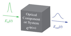
Since we are interested mainly in the effects of dispersion, we assume there is a uniform amplitude frequency dependence, such that the same intensity of light is transmitted at each frequency. The system may then be described simply by the optical phase φ it imparts to each frequency ω of a light wave.

To describe the pulse of light, we consider a simplified mathematical description of the pulse at wavelength λ traveling in direction z,

,     (1)

where e_in(t) describes the temporal shape of the pulse, k = 2π/λ is the wave propagation constant, and ω₀ = 2πc/λ is the angular frequency of the wave with c the speed of light (3×10⁸ m/s). It is assumed that e(t) varies in time much more slowly than the frequency ω₀ of the wave. The subscript “in” identifies that the pulse is heading into the system of interest.

The mathematical procedure for calculating the output pulse E_out(t) is described in the APPENDIX to this Technical Note. While the method can be used for any phase function φ(ω), little insight is gained by simply turning this crank on a computer. Often the pulse spectrum is sufficiently narrow and the phase function φ is relatively smoothly varying over this narrow spectral range. Then φ at frequency ω can be well approximated by a Taylor series expansion about the central frequency ω₀ according to

.     (2)

Expanding φ in this way not only simplifies the math, but also enables helpful physical interpretation of the physics of dispersion. The first term is just a constant phase and has no impact on the measured intensity of light transmitted through the system. The coefficient of the second term dφ/dω = φʹ has units of time and is called the group delay time. We will see why shortly. The coefficient of the third term d²φ/dω² = φʺ has units of time squared and is called the group delay dispersion, or GDD [1].

A simple example – a gaussian pulse shape:

Much insight on how dispersion affects a pulse can be gained using the simple approximation of phase in (2) and a gaussian pulse shape. The gaussian pulse can be described by

,     (3)

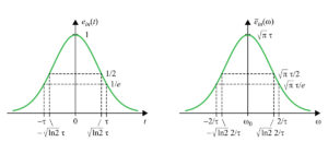
where τ is a measure of the pulse width. The spectrum of this gaussian pulse, denoted ē_in(ω), also has a gaussian profile, and can be written

.     (4)

These two profiles are illustrated in Figure 2, where both the 1/e and half-maximum widths are identified. The pulse has a full width at 1/e of 2τ, whereas the spectrum has a full width at 1/e of 4/τ. So the broader the pulse is, the narrower its spectrum is.

Using the method described in the APPENDIX, we can now calculate the full output pulse as

,     (5)

where

     (6)

is a time-dependent frequency of the output pulse. In (5) and (6) we have defined the following quantities:

     and     .     (7)

C is called the chirp parameter and τ_C is the chirped pulse width. Looking closely at (5) – (7) we observe four fundamental ways a pulse is affected by dispersion.

Consequences of dispersion for a pulse:

1. The pulse is delayed.

From (5) it is clear that the output pulse also has a gaussian shape, but t has been replaced by t – φʹ in the time dependence. Referring to Figure 3, physically this substitution means that the pulse emerging from the optical system is no longer centered at time t = 0, but is now centered at time t = φʹ. In other words, it has been delayed in time by φʹ. The first derivative φʹ is called the group delay time because it is the amount of time the group of frequency components that form the pulse are delayed by the optical system.

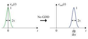
Note that on a time graph like those shown in Figure 3, the convention for interpreting the orientation of the pulse is as follows:  if an observer sits at the value of z at which the pulse shape e(t) is evaluated, then the observer sees the value of e(t) shown on the plot after waiting a time t on the plot. Thus the observer sees the left side (i.e., earlier times) of the plotted pulse shape first.

2. The pulse is broadened.

Again referring to the exponent of the gaussian function in (5), the width of the output pulse is now determined by τ_C instead of τ. The output pulse is broader than the input pulse by a factor of √(1 + C²). Since C is proportional to the GDD parameter φʺ, then the higher the absolute value of φʺ, the more the pulse is broadened. Figure 4 illustrates a pulse that is delayed and broadened by the group delay time and GDD, respectively.

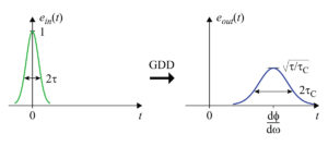
Figure 5 shows examples of how the output pulse width of a gaussian pulse increases as a function of the GDD. In the graph on the left, five initial pulse widths ranging from 10 to 400 fs are considered for GDD values ranging from 0 to 10,000 fs². Note the smaller the initial pulse width, the lower the GDD required to broaden the pulse substantially. For a 400 fs pulse, even 10,000 fs² has almost no effect on the pulse width.

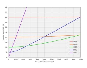
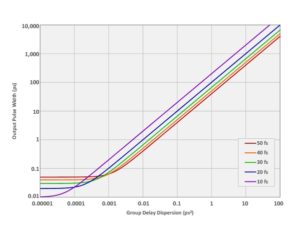
The graph on the right considers higher values of GDD to demonstrate how much dispersion is required to stretch or compress a pulse with a width of 10’s of fs in a CPA system. Stretching to 100 ps requires about 1 ps² = 10⁶ fs² of GDD, whereas to stretch to 1 ns requires about 10 ps² = 10⁷ fs².

3. The pulse is squished.

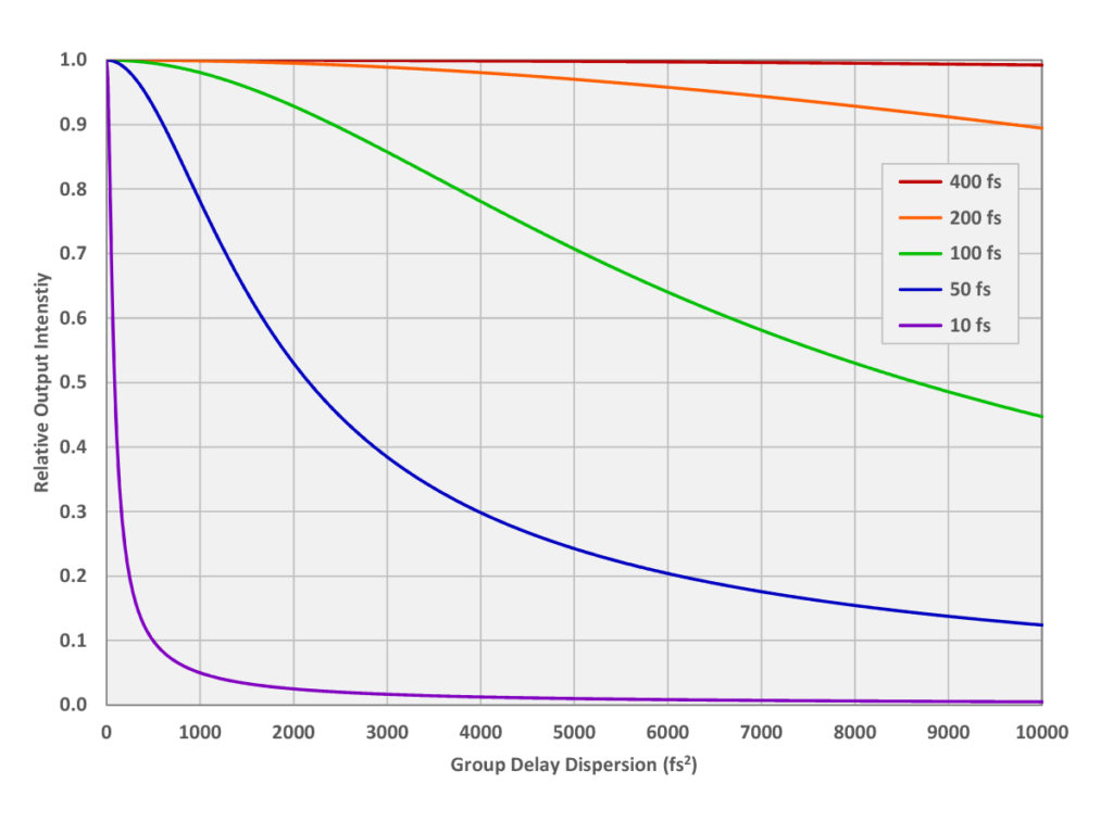
According to (5) the amplitude of the dispersed electric field is “squished,” or reduced, by a factor of √(τ/τ_C) relative to the amplitude of the input pulse. This effect is also illustrated in Figure 4. Since the intensity of a light wave is proportional to |E(t)|², then the output pulse peak intensity is a factor of τ/τ_C smaller than that of the input pulse. As an example, Figure 6 shows how the relative intensity depends on GDD for the same initial pulse widths and range of GDD values shown in the graph on the left in Figure 5.

4. The pulse is chirped.

Chirp refers to a signal in which the frequency increases or decreases with time. We expect the dispersed pulse to be chirped because the mechanism by which it is broadened is in fact different frequency components being delayed by different times as it is transmitted through the dispersing component or system. For a gaussian pulse, the chirp is described by the time-dependent frequency ω(t) in (6). This is an example of a linear chirp, since the frequency is directly proportional to time.

Figure 7 illustrates an unchirped initial pulse (left) as well as chirped pulses resulting from both positive and negative GDD (center and right, respectively). For illustration purposes the frequency relative to the pulse width shown here is much lower than typical in most real systems.

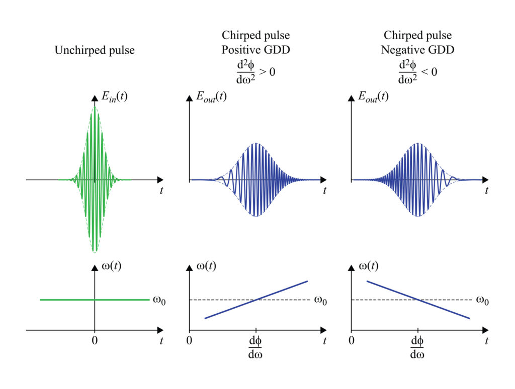
Notice that for φʺ > 0 (positive GDD) the frequency increases at later times. Thus a fixed observer sees lower frequencies in the chirped pulse arrive first. Loosely, we say the “red” part of the pulse arrives ahead of, or leads, the “blue” part. For φʺ < 0 (negative GDD) the red part of the pulse lags the blue part.

Dispersion from a pair of gratings:

In the Technical Note “Temporal Dispersion” we found the temporal dispersion parameter for diffraction of light off of a pair of parallel gratings,

,     (8)

where m is the order of diffraction, λ is the wavelength of light, f is the grating frequency, θ_m is the angle of diffraction, and the subscript “⊥” denotes that the grating separation s is measured along the direction normal to the grating surfaces. This physically useful parameter can be interpreted as follows:  for each meter of separation s between two parallel gratings, the difference in propagation delay time dτ between two wavelengths of light separated by dλ can be approximated by the expression on the right side of (8) multiplied by dλ.

We may also directly relate D to GDD. Using the chain rule of calculus, we can see

,     (9)

where we have used the delay time τ = dφ/dω. From (9), we may now directly relate D to GDD as

     and     .     (10)

Keeping careful track of units and simplifying, we may use the following conversion relations

     and     ,     (11)

where s is in meters and λ is in nm. Note that D and φʺ have opposite signs. Combining (8) and (10), we may directly write the GDD in terms of grating parameters as

.     (12)

For a simple parallel grating pair, the GDD is always negative. In other words, the blue part of a pulse leads the red part. In most CPA systems pulses are stretched using an arrangement that provides positive dispersion, and then compressed using the negative dispersion from a parallel grating arrangement.

Using (12), we may plot an example of the GDD as a function of the angle of incidence for a certain wavelength. Figure 8 shows how the GDD of the –1^st order depends on angle of incidence at 800 nm for three different grating frequency values.

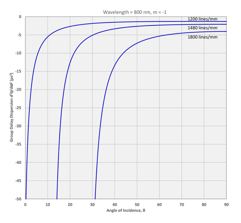
The absolute value of the GDD is larger for higher grating frequencies at a given angle of incidence. Furthermore it increases rapidly at smaller incidence angles, as the diffraction angle approaches –90º.

APPENDIX – Mathematical treatment of pulses:

As explained above, we can describe the pulse in terms of its electric field according to (1). We are only concerned with how the scalar electric field E(t) depends on time t. We ignore the polarization and transverse beam properties of the pulse, equivalent to assuming a nearly perfect plane wave with simple (e.g., linear) polarization. In (1) E(t) is assumed to be a real quantity, obtained by taking the real part of the right-hand side of this equation (the “real part” notation is suppressed).

Since the optical component or system imparting dispersion to the pulse is characterized by its frequency response, we must somehow transform (1) into a description of the electric field in terms of frequency, not time. We can think of the pulse shape e_in(t) as a superposition of many monochromatic plane waves, each at frequency ω = ω₀ + Ω, and each with an amplitude ē_in(Ω) = dΩ/2π. Writing this superposition as an integral,

.     (13)

Note that (13) has the mathematical form of an inverse Fourier transform. Therefore ē_in(Ω) must be the Fourier transform of e_in(t), or

.     (14)

In words, e_in(t) is the initial, slowly varying pulse shape, and ē_in(Ω) is the initial spectrum of the pulse. The temporal and spectral descriptions of the pulse form a Fourier transform pair. Therefore, if the pulse is very narrow in time, the spectrum must be very broad, and vice versa.

For each value of Ω = ω – ω₀, we know the wave accumulates an additional phase φ(ω = ω₀ + Ω) as it passes through the dispersing component or system. Therefore the output spectrum is simply

.     (15)

The output pulse shape is the inverse Fourier transform of the output spectrum, or

.     (16)

The full output pulse electric field is then simply

.     (17)

To summarize, the procedure for calculating the output pulse E_out(t) from the input pulse E_in(t) is as follows:

1. take the Fourier transform of the input pulse shape e_in(t) according to (14);
2. multiply the spectrum ē_in(Ω) from a. by exp(iφ) using φ(ω = ω₀ + Ω) according to (15);
3. take the inverse Fourier transform of the output spectrum ē_out(Ω) from b. according to (16), and then put it in the form of the full output pulse according to (17).

This prescription is valid for any phase function φ. However, often the pulse spectrum is sufficiently narrow and the phase function φ is sufficiently smoothly varying over this narrow spectral range that (2) is a reasonable approximation and can greatly simplify the math and offer helpful intuition, as we see above for the gaussian pulse shape example.

References and end notes:

[1]  Often group delay dispersion (GDD) is confused with group velocity dispersion (GVD). These two quantities are closely related, as both describe the second-order dependence of a wave’s properties on frequency. GVD specifically refers to frequency dependence of a wave’s propagation constant. It makes sense to talk about GVD in a system in which a wave is propagating over some distance, such as a block of glass with a frequency dependent index of refraction or an optical fiber. In this case GDD – the dispersion or frequency dependence of the time delay—is simply the GVD multiplied by the length traveled. However in the case of an optical component or system that imparts dispersion in a more complicated way, it doesn’t make sense to describe dispersion in terms of GVD. We only see the overall group delay, or, in terms of dispersion, the overall group delay dispersion, GDD.

[2] See PGL Technical Note “Temporal dispersion”